The following steps will walk you through the process of creating a graph. Please note that if you have not already, you will need to enable the “Counts” views as described in the “Enabling the “Counts” Views” section of this document.
1. Start and log into TOXICALL®
2. Select the network database search window icon.
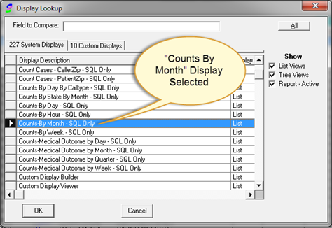
3. With the network database search window open, select the “Display” 3-dot button and update the display to the desired “Counts” view to graph. In this example we will use “Counts By Month” display.
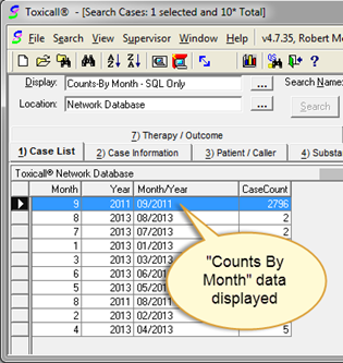
4. Enter any search criteria desired and press search to display the requested data.
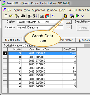
5. With
your data showing from the Counts search click on the  Icon to open the graph configuration
window.
Icon to open the graph configuration
window.
6. The “Graph Configuration Settings” window will open.
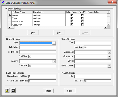
Below is a list describing each field and its purpose.
Graph Settings:
•Style – This is a list of different types of graphs that can be used
•Tab Label – Labels the data produced in an excel spread sheet along with the graph
•Graph Title – The title of the Graph
•Legend – This can be configured to either show the legend or not. It also determines the legends orientation if one is used.
X-Axis settings:
•Title - The title of the X-Axis on your graph
•Alignment – The position of the X-axis title. (TOP and BOTTOM is currently NOT supported. If you select either one of these options you will receive an error when the graph is generated.)
•Orientation - The angle at which the X-axis text label will be displayed
•Offset – The amount of space the label will appear from the graph, (recommend 100)
•Value Column – The value to graph on the X-Axis
Y-Axis:
•Title – The title of the Y-Axis
 - Opens a saved graphing
configuration
- Opens a saved graphing
configuration
 - Saves a graphing
configuration.
- Saves a graphing
configuration.
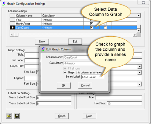
7. In the “Column Settings” area choose a column to graph by double clicking the entry. In the “Edit Graph Column” window, check the “Graph this column as a series” check box and provide a series name. The below image can be used as a guide.
 .
.
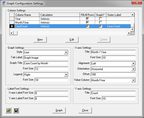
8. Next you will fill in the remaining settings as desired. The following image shows a completed example.
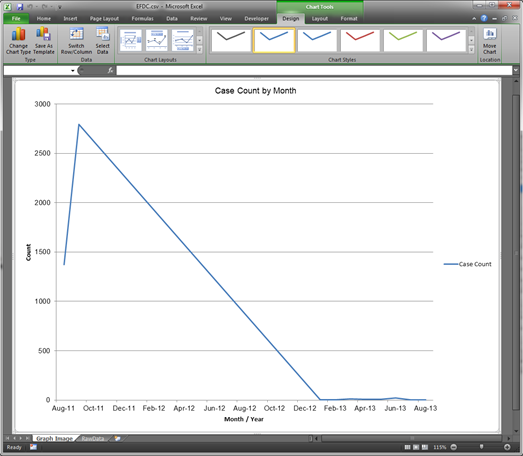
9. Once you have the settings desired entered, press the “Graph” button to generate the graph. The following image is the generated graph.
10. At this point the graph is saved as a temp .CSV file. If you would like to save the graph as a .xls or .xlsx Excel workbook in a specific location, select “File” then “Save As” to provide a unique name, extension, and save location.